June 2016 v2
For this project, I selected my home region, Ann Arbor, Michigan. Ann Arbor is home to the University of Michigan and bounded by the Detroit exurbs on the east and by farmland and parks to the west. I loaded and performed simple cleaning on the dataset but as you will see, I got curious about the editors and ran off looking for more information about that.
I chose three expanding areas for my early data acquisition, expanding outward from my house. Although I was able to extract smallarbor.osm directly from the OSM export function, medarbor.osm and annarbor.osm had to be pulled from overpass. All datasets, including the sampled set generated for the assignment, are stored in the /osmfiles subdirectory. Early audits and data exploration were made and tested on the smallest set (smallarbor.osm) and then expanded outward. Final code all points to the main annarbor.osm dataset.
I leveraged a number of the routines developed during the course exercises - and these do include functions that were provided by the course team for utility work. Based on suggestions in the project rubric, I inspected the contributors and the street names in the file while assessing the raw XML data. Detailed code for the XML audit and export to sqlite are in 01audit-export.py. All tables were exported to CSV after they were generated for later reference.
This audit came straight out of the exercises - poking around in Ann Arbor didn't really reveal any intriguing new issues other than some over-abbreviation. I adjusted the code in order to include some typical Michigan road-names (Eight Mile really is a valid road) and built a list of proposed namings. Rather than write the changes back to my source data, I created a small table in SQL for later reference and repair.
Phone numbers were also formatted very inconsistently. I handled these differently - I moved all the nodes-tags over to SQL and then extracted those whose keys were 'phone' back to a data frame for manipulation. The pandas regex functionality allowed me to quickly break phone numbers apart from their punctuation. I reassembled them and then replaced (all but one that didn't fit) consistently-formatted numbers in the database. It's one of the routines in usingsql.py
Over each table, I ran:
cur.execute("SELECT COUNT (*) FROM %s;" % table_name)
and
cur.execute('PRAGMA TABLE_INFO({})'.format(table_name))
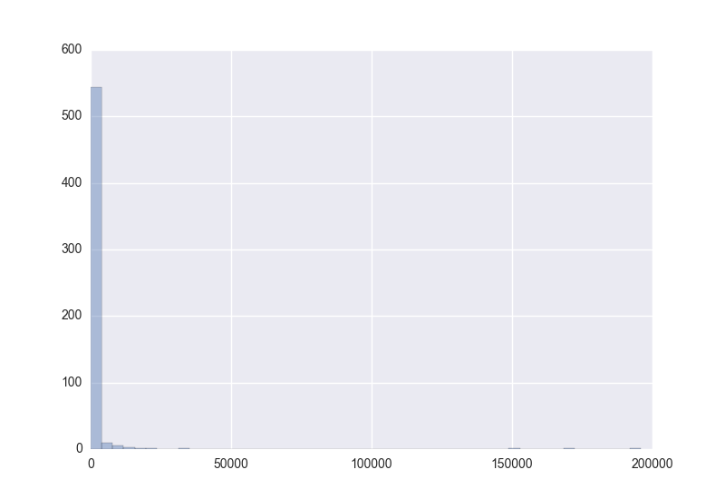
For the sake of exercising both XML and SQL-fu, I pulled the list of contributors from the annarbor.osm file and found:
This was really intriguing. So the overwhelming majority of users contribute only one edit, but a tiny number contributed hundreds of thousands! The biggest obstacle I encountered during this exercise was the Python unicode trap. I had to add the codecs module and convert in and out of UTF-8 in order to get some editors' names with unusual characters to process correctly.
image:
Most prolific editors:
{'Gone': 170997, 'woodpeck_fixbot': 150070, 'DougPeterson': 195860}
Account for 61.823685523 percent of edits.
I went way, way, way down a rabbit hole on this: for more analysis, check the Appendix.
I executed this over each of the tag tables:
"SELECT COUNT(*) AS ct, key FROM {}
                             GROUP BY key ORDER BY ct DESC LIMIT 15;".format(table_name)
nodes_tagsct key0 4131 highway1 3348 power2 1891 name3 1784 created_by4 1537 amenity5 462 street6 457 ele7 432 housenumber8 404 barrier9 388 feature_id10 385 shop11 373 ref12 314 railway13 312 created14 304 man_madeways_tagsct key0 44459 highway1 27479 name2 22299 county3 22250 cfcc4 20809 reviewed5 20181 name_base6 18044 name_type7 16055 zip_left8 15513 zip_right9 9166 building10 7141 source11 6848 service12 4718 oneway13 3761 amenity14 3621 NHD:ComID
This little routine gave me short tables of common tags. unsurprisingly, "highway" and "name" are really popular for both nodes and ways - a little more oddly, there were a great number of 'power' nodes. Looking further revealed that someone has planted every single power pole in the city of Ann Arbor into OSM.
I decided to follow up on the tag, 'cfcc.' What was that?
SELECT COUNT(*) as ct, value FROM ways_tags WHERE key = 'cfcc' GROUP BY value ORDER BY ct DESC LIMIT 10;
That's a lot of A41.
Google revealed that CFCC are ways of classifying roads. A41s are 'Primary road without limited access, US highways, unseparated.' The data almost certainly came from the original census data.
Who wrote all that?
SELECT COUNT(*) as ct, ways.user FROM ways JOIN ways_tags ON ways.id = ways_tags.id
                            WHERE ways_tags.key = 'cfcc' GROUP BY ways.user ORDER BY ct DESC LIMIT 10;
Ah. The very early bots placing census data. Makes perfect sense.
If I were to tackle this data set more, I'd pull the relations in and start to play with them. I think that's where the history starts to get interesting. I also think we could learn more about who are custodians of what kind of map data and start to build human community alongside this interesting virtual one.
I had wondered whether finding ways with higher point density would help identify trails for non-motorized vehicles. Pathways that are more amenable to runners and cyclists might be teased out if we were able to establish that a particular route was defined at a high level of detail.
This depends, however, on the assumption that slow-moving GPS devices were used to identify and track trailways. I'd start by pulling each Way and calculating point density by calculating the average distance between each pair of closest nodes in the Way. This could then be tied back to a list of Ways and checked against what we already know about local roads and trails. If there's a clear link between high point density and some known runner-friendly pathways, we could then try comparing high-point-density ways to others in the set and seeing whether the correlation is helpful.
I got really interested in the editors who had contributed to the project.
So, I got curious. A small number of editors make a large number of edits. I wanted to learn more. I started by making a relatively simple image, plotting every data point onto a simple map. There are so many nodes, however, that I had to make them very, very transparent in order to show anything useful.
The code leverages the matplotlib Basemap library. The following maps were generated with very similar code. The source is in 05mapping.py
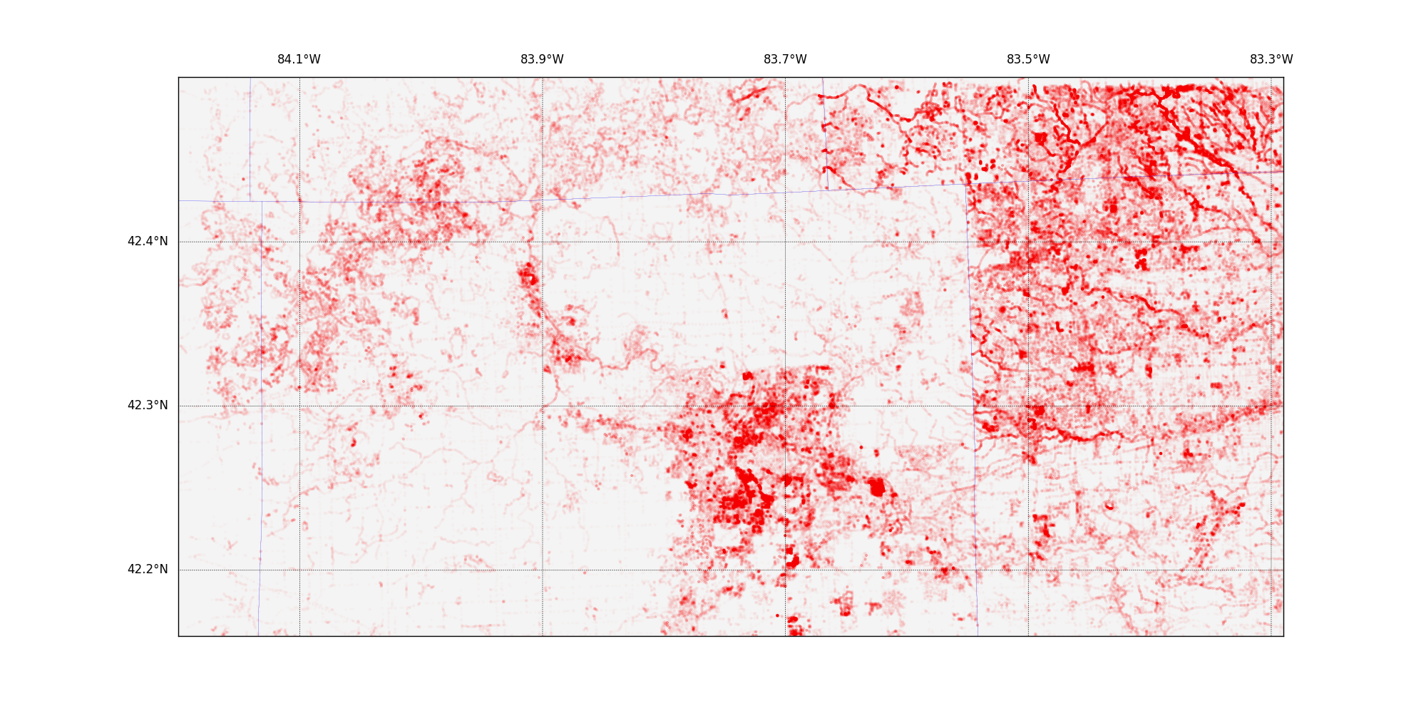
I really enjoyed looking at this plot - it is stripped of all tag information - all you can see is that there are many more nodes in some places than in others: roads, rivers, and electricity poles are all the same. In this plot and in the two other maps shown, county boundaries are shown in thin blue lines to help you orient from one map to the next. The map immediately shows how land use (and density of interesting information) changes over the line between Ann Arbor's Washtenaw County and the Detroit area's Wayne County to the east. I found the visual impact striking.
A common tag was 'version.' After I saw this map, I expected to find that data in the central urban area would be most likely to have high version numbers as it was updated and edited in a dynamic environment. So I redrew the map so that it showed those nodes with the highest version number in darker blue.
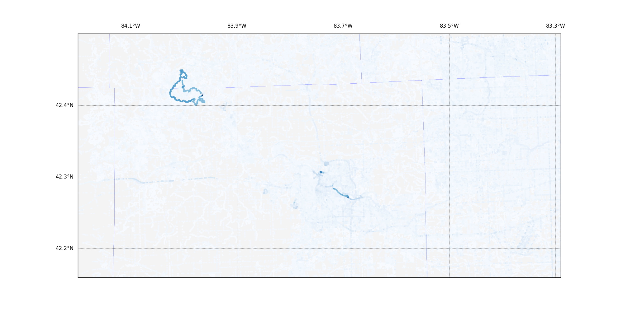
That was entirely unexpected.
Way off in the northwest corner of the search area, it turns out that a mountain bike trail called the Potawatomi Trail has had as many as 34 different versions of its nodes, ways, and/or relations. (I did not include relations in this analysis but went back and looked when I found this.) Now, I've wiped out on almost every root of the 17 miles of this trail, but I'm baffled that it has had so much more TLC than any other part of the region.
If you compare this to the red map above, you'll note that there isn't a markedly high point density in the area of the trail. It's just that what points are there have incredibly high version numbers.
So I got more curious. Let's see again who the key editors for the Ann Arbor map are:
"SELECT COUNT(*) AS ct, user FROM nodes
GROUP BY user ORDER BY ct DESC LIMIT 15;", con)
Doug Peterson has been mighty busy for a guy who isn't a robot. I created the userindex
to simplify mapping each of these names to a color. I also decided to try to create
a plot that might indicate whether these guys or gals seem to work on different parts
of the county. I created a table that calculated the mean latitude and longitude
values for each of the editors and plotted on a grid with the point size indicating the
number of edits.
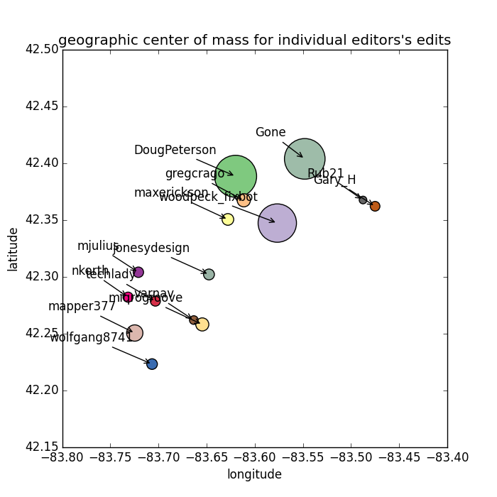
That was actually really disappointing. It didn't tell me much, but you, dear reader, should hang onto it, because it color-keys the editors for the next exploration.
Instead of a crude center of mass, I decided to go ahead and plot each point the
fifteen biggest editors hand touched and give them each a color. It's the same color
as in the picture above.
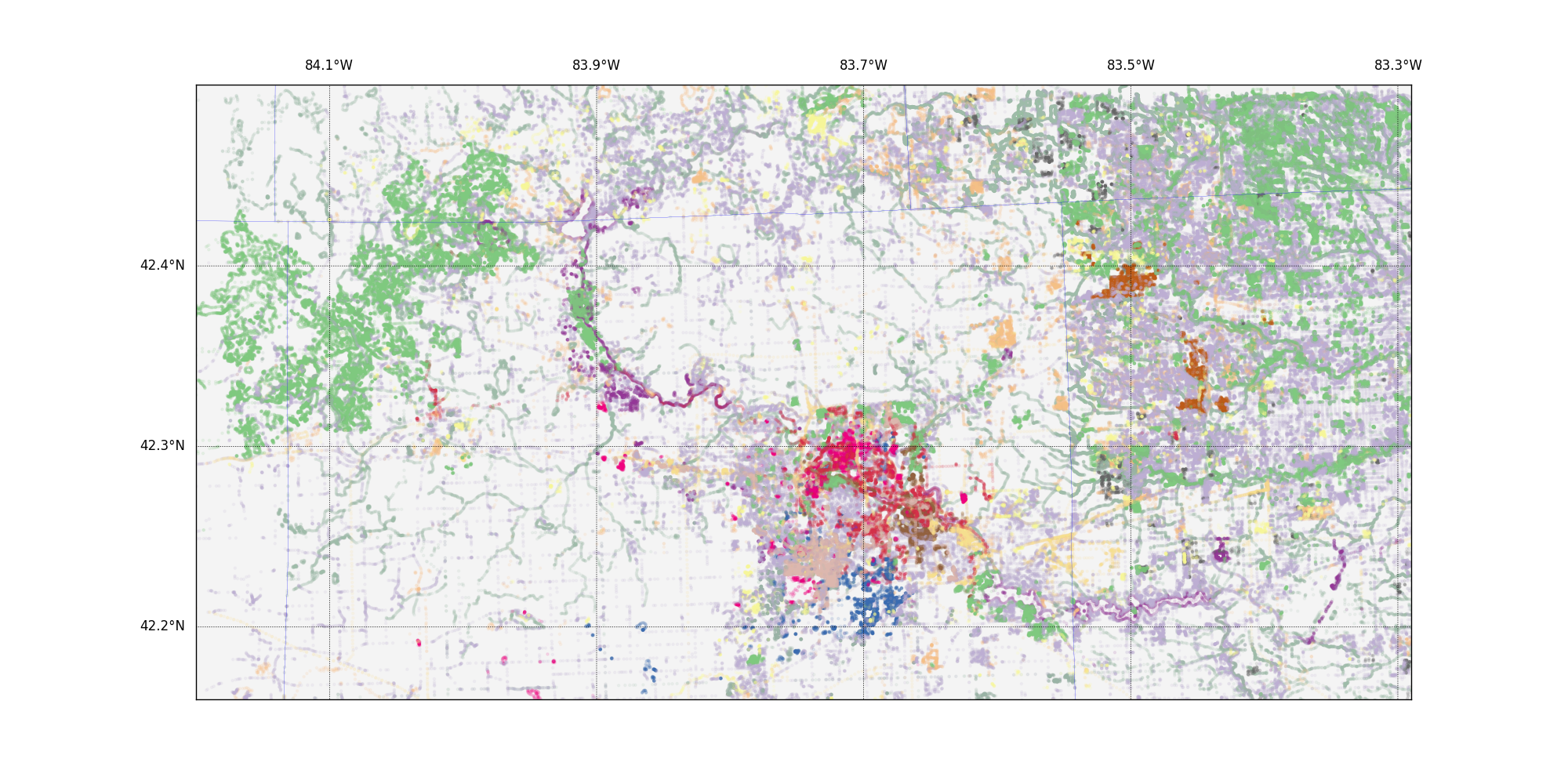
And it turns out that our friend Doug has been concentrating his efforts in the parkland out west of the city. What if we constrain the points to only those in the general vicinity of the Poto?
SELECT COUNT(*) as count, user from nodes
        WHERE (lat < 42.46 AND lat > 42.39 AND lon > -84.035 AND lon < -83.96)
        GROUP BY user;
...and there's Doug. Big-time. As it turns out, the OSM site tells us a lot that we were intuiting here: The Poto's relations data shows a 7-year editing effort that includes many, many update sets. He's been key to these edits and has been on the spot every time the trail moves, or a park bench is put in. In case you are interested, the history is here:
https://www.openstreetmap.org/relation/48886/history#map=13/42.4250/-84.0161